要点速览
- AV 此前仅支持带 confidence head 的 DSpark;在线拟合估计器让 EAGLE、MTP、DFlash 等免重训接入 AV。
- 估计器是逐位置逻辑回归:特征为草稿最可能 token 的 logit(q_max),共享斜率+逐位置截距共 K+1 参数,由目标模型的接受/拒绝标签在线拟合。
- 选定特征 logit(q_max) 无损且均衡(AUC 0.8336、ECE 0.0100):AUC 优于训练 head,校准略逊但排除首位置后基本打平。
- 拟合用 IRLS 每 N 步重解一次,期间只累积梯度与 Hessian,内存上界 O(K²);共享斜率+步长阻尼缓解深位置标签稀疏。
- 端到端性能与 confidence head 大致相当;MiMo+DFlash 上 AV 在 7 个并发中的 5 个位于吞吐-交互前沿。
解决什么问题
vLLM 的自适应验证(AV)需要逐 token 的接受概率估计来决定裁剪哪些草稿 token,但此前只有自带 confidence head 的 DSpark 草稿模型可用。EAGLE、MTP、DFlash 及部分 DSpark checkpoint 缺少该头部,补上意味着重新训练草稿模型,对已在线服务的大量既有 checkpoint 并不可行。此外,AV 的预算决策要求预测概率针对具体模型对与负载校准,直接拿草稿模型自身的置信度当接受概率会失准。
核心思路
核心做法是在草稿模型侧加一个轻量的逐位置逻辑回归:以草稿分布最可能 token 的对数几率 logit(q_max) 为唯一特征,用一个全位置共享的斜率 ω 和每个草稿位置一个截距 β_i(K 个位置的草稿模型只需 K+1 个参数)预测接受概率。系数不做离线训练,而是在服务过程中用目标模型验证时自然产生的接受/拒绝标签持续在线拟合。具体用 IRLS 对 log-likelihood 损失做二阶泰勒近似,每 N 步解码累积梯度与 Hessian 后解 H·Δθ=−g 更新系数,内存上界 O(K²)。为应对深草稿位置标签稀疏,斜率全位置共享,且每步更新按证据量 n/(n+常数) 阻尼。在 vLLM 中通过 enable_adaptive_verification 开启,无 confidence head 的草稿模型会自动选用该估计器。
关键要点
- 特征选择:logit(q_max) 的胜出 — 估计器只用一个标量特征——草稿分布中最可能 token 的对数几率 logit(q_max)。在四个评估轴(无损、AUC、log-loss、ECE)上,它兼顾区分度(AUC 0.8336)与校准(ECE 0.0100),综合优于 top-2 margin、熵、q_max 直接使用等候选。它与待估计的接受概率同为 log-odds 尺度,也是自然的选择。
- 无损性是不可协商的底线 — 基于 q_sampled(被实际采样 token 的概率)的特征 AUC 更高(0.8553/0.8554)却不能用:按它裁剪会让「位置 i 是否验证」依赖于 x_i 本身,存活的草稿不再服从分布 q。标准拒绝采样以 min(1, p/q) 接受 token,前提是草稿确实从 q 采样;基于 q_sampled 裁剪会把输出分布偏向草稿的高置信 token,破坏推测解码的精确分布保证。
- AUC 管局部排序,ECE 管全局预算 — AV 的裁剪用 topk 选草稿 token,AUC 保证更可能被接受的草稿优先入选(局部排序正确)。预算决策则把预测概率沿位置求和、除以实测成本表取 argmax,ECE 保证估计的接受 token 数贴合现实(全局校准)。log-loss 同时惩罚错误的自信并奖励校准,是拟合优化的目标。
- 对比训练 confidence head:深位置反超 — 整体上估计器 AUC 与 log-loss 更优、ECE 略逊;排除首草稿位置后两者校准几乎打平,估计器 AUC 领先扩大到 +0.0278。confidence head 只在首位置更强,估计器从第二位置起领先并在末位扩大到 0.08 AUC。由于存活概率是累积乘积、首位置得分最高而很少被预算裁掉,估计器的优势恰好在裁剪发生的地方,这解释了它端到端性能能追平 confidence head。
- 在线拟合:IRLS 与 O(K²) 内存 — 系数在服务期间持续重拟合:每 N 步解码为一个轮次,期间只累积 Hessian 和梯度,轮末解 H·Δθ=−g 后更新,内存上界 O(K²),远低于存原始标签的 O(N×B×K)。训练样本只取到首次拒绝为止的草稿 token,因为只有它们被目标模型明确标注了接受/拒绝。
- 斜率与截距的分工 — 固定模型对、变负载时,斜率几乎不动(0.51–0.55,与草稿熵相关系数 −0.08),而首位置截距与熵强相关(r=−0.89),从可预测负载的 ~0.5–0.6 跌到最难负载的 0 以下。跨模型对时斜率在 0.45–0.59 之间、对内很紧。解读:斜率度量草稿模型「知道自己何时正确」的程度,是模型对与采样方法的属性;截距吸收随深度和负载变化的基线接受率,沿两个轴移动。
- 两个设计决策对抗深位置标签稀疏 — 深草稿位置接受率低,一轮内可能得不到足够标签。其一,斜率全位置共享,避免逐位置斜率因数据稀薄产生噪声更新(预测对斜率误差远比截距敏感),实测共享只损失 0.0002 AUC 和 0.0003 log-loss。其二,步长阻尼用 n/(n+常数) 按支持证据量缩放每个系数的更新,让标签少的位置保守移动。
- 基准表现与局限 — 三个原本无法使用 AV 的 checkpoint(MiMo-V2.5-Pro-FP4 + DFlash、Inkling-NVFP4 + MTP、Muse-Glimmer-30B + DFlash2)在相同推测长度下开启 AV 后各数据集均有吞吐增益;MiMo 上 AV 在 7 个并发中的 5 个位于吞吐-交互前沿。局限:目标模型注意力后端必须支持变长验证(与 DSpark AV 相同);MTP/EAGLE 这类自回归 speculator 为可能被裁掉的 token 付出的草稿成本占比更高,收益不如 DFlash/DSpark。
关键数据
| 指标 | 数值 | 条件 |
|---|---|---|
| 上线特征 logit(q_max) 的评估指标 | AUC 0.8336 / log-loss 0.4284 / ECE 0.0100 | DeepSeek-V4-Flash + DSpark,约 4.5M 标注草稿(temp=1, top-p=0.95, conc=64,五个数据集,未开 AV) |
| 训练 confidence head 的评估指标(参照) | AUC 0.8191 / log-loss 0.4449 / ECE 0.0052 | DeepSeek-V4-Flash + DSpark,同一标注集 |
| 排除首草稿位置后估计器相对 head 的优势 | ΔAUC +0.0278 / Δlog-loss −0.0323 / ΔECE +0.0013 | DeepSeek-V4-Flash + DSpark |
| 估计器在末位置的 AUC 领先幅度 | 0.08 AUC | DeepSeek-V4-Flash + DSpark,7 个推测 token,4.47M 标注草稿 |
| q_max 不拟合直接当概率用的校准偏差 | 平均预测 0.784 vs 实测接受率 0.723;ECE 0.0736 vs 0.0100(约 7 倍) | DeepSeek-V4-Flash + DSpark 标注草稿集 |
| 在线拟合的内存上界 | O(K²),对比收集原始标签的 O(N×B×K) | 每轮 N 步解码,期间累积 Hessian 与梯度;K 为草稿长度 |
| 共享斜率的精度代价 | 0.0002 AUC / 0.0003 log-loss | 斜率全位置共享 vs 逐位置独立拟合的实测差 |
| 斜率随负载的变化范围 | 0.51–0.55(与平均草稿熵相关系数 r=−0.08) | DSV4-Flash + DSpark 在五个负载上独立拟合 |
| 首位置截距与草稿熵的相关性 | r = −0.89;截距从 ~0.5–0.6 降到 0 以下 | DSV4-Flash + DSpark,五个负载 |
| 斜率跨模型对的范围 | 0.45–0.59(单个模型对内保持紧凑) | DSV4-Flash+DSpark、MiMo-V2.5-Pro-FP4+DFlash、Inkling-NVFP4+MTP、Muse-Glimmer-30B+DFlash2 四个模型对 |
| AV 位于吞吐-交互前沿的并发比例 | 5/7 | MiMo-V2.5-Pro-FP4 + DFlash,固定推测长度扫描 vs 最大长度 AV |
| 特征评估所用标注草稿规模 | 约 4.5M 条 | DeepSeek-V4-Flash + DSpark 服务期间收集,temp=1, top-p=0.95, conc=64,未开 AV,覆盖 SPEED-Bench 2k 低/高熵、GSM8K、HumanEval、MT-Bench 五个数据集 |
“| **logit(*q*<sub>max</sub>) (shipped)** | **yes** | **0.8336** | **0.4284** | **0.0100** |”
“| **trained confidence head** | **yes** | **0.8191** | **0.4449** | **0.0052** |”
“| **Δ (estimator − head)** | **+0.0278** | **−0.0323** | +0.0013 |”
前置知识
推测解码基本流程:草稿模型提案、目标模型验证、拒绝采样 min(1, p/q) 保证输出分布无损 · vLLM 自适应验证(AV)的裁剪与预算机制(建议先读 2026-08-14 DSpark AV 博文) · 逻辑回归与 logit(log-odds)变换 · 分类评估指标:AUC(区分度)、log-loss、ECE(校准) · 牛顿法/IRLS(迭代重加权最小二乘)、梯度与 Hessian · 常见草稿模型类型(DSpark、EAGLE、MTP、DFlash)及 confidence head 的有无
术语表
Adaptive Verification (AV): 自适应验证:推测解码中先裁剪掉预测接受概率低的草稿 token 再跑目标模型前向以省算力,大 batch 计算受限时收益最大Confidence head: 置信头:草稿模型上逐位置的小型线性层,作为二分类器预测目标模型是否会接受该 token,需随草稿模型一起训练logit(q_max): 草稿分布中最可能 token 的对数几率(log-odds),估计器的唯一特征,反映草稿模型对自身预测的置信程度IRLS: 迭代重加权最小二乘:对 log-likelihood 损失做二阶泰勒近似后,解 H·Δθ=−g 的牛顿步来拟合逻辑回归系数AUC: ROC 曲线下面积:随机选一个被接受草稿比被拒绝草稿得分更高的概率,衡量排序/区分能力,0.5 为随机ECE: 期望校准误差:按预测概率分箱后衡量箱内预测均值与观测频率的加权偏差,衡量校准程度,越低越好Step damping: 步长阻尼:用 n/(n+常数) 按支持证据量(被标注草稿数 n)缩放系数更新,让标签稀少的深草稿位置更新更保守Survival probability: 存活概率:置信概率沿草稿位置的累积乘积,决定 topk 裁剪中哪些草稿 token 入选预算
Adaptive Verification Without a Confidence Head
TL;DR
Confidence scoring is now supported for all draft-model-based speculator types. In the absence of a confidence head, an online-fitted estimator derives a feature from the drafter's logits to predict the target model's probability of accepting it, which is used directly as a confidence score for Adaptive Verification. The estimator's coefficients are continuously fitted, adapting to the incoming data traffic. This feature landed in PR #52228, and is enabled with enable_adaptive_verification for draft models without a confidence head.
Background
vLLM's Adaptive Verification (AV) enables verification of a subset of the drafted tokens during speculative decoding. Draft tokens with low probability of acceptance are trimmed from the batch before running the target model's forward pass, saving on compute. This optimization is particularly beneficial while serving large batch sizes, because in that regime the GPU becomes compute-bound. See this vLLM blog post for more details.
AV needs a per-token estimate of acceptance probability, which is why, until now, it only supported DSpark drafters. DSpark models often ship with a confidence head: a small linear layer over the drafter's hidden state for each position, trained as a binary classifier for "will the target accept this token?"
Problem
Draft models that lack a confidence head, such as EAGLE, MTP, DFlash, and some DSpark checkpoints, miss out on AV entirely. To use it, these drafters need a per-token acceptance estimate, and adding a confidence head means retraining the drafter, which isn't an option for the many existing checkpoints that people already serve.
Prior Work
Using the drafter's own confidence as a proxy for acceptance is well established. EAGLE-2 showed that EAGLE's draft probabilities closely track acceptance rates, and used them to grow and rerank a dynamic draft tree. Draft & Verify and several follow-ups stop drafting once the drafter's probability falls below a fixed threshold. SpecDec++ instead trains a dedicated acceptance-prediction head, similar in spirit to DSpark's confidence head. In each case, the mapping from draft confidence to acceptance is either used as-is or learned offline.
AV needs more than a good ranking. Its budget decision sums predicted acceptance probabilities and weighs them against measured costs, so the predictions must be calibrated for the specific model pair and workload being served, which is what the online-fitted estimator in the next section provides.
Solution: Online-Fitted Acceptance Estimator
We added a lightweight logistic regression that estimates each draft token's acceptance probability from a single scalar derived from the draft distribution, the log-odds of the drafter's most likely token. It has one shared slope and one intercept per draft position, so a K-token drafter needs a total of K + 1 parameters. Those parameters are fitted online from the accept/reject decisions the target model already produces during normal verification. Any existing draft checkpoint gets AV for free.
The rest of this section covers the two halves of the design: what quantity the estimator scores, and how its coefficients are fitted during serving.
Scoring the Distribution
The confidence score for a given draft token is estimated using a per-position logistic regression:
$$ p = \sigma\big(\omega \cdot \text{logit}(q_{\max}) + \beta_i\big) $$
where ω is the fitted slope shared across all draft positions, βi is the fitted per-position intercept, and q is the draft distribution. The alternate log-odds form makes the relationship clear:
$$ \text{logit}(p) = \omega \cdot \text{logit}(q_{\max}) + \beta_i $$
logit(qmax) is the estimator's feature, and is the log-odds of the draft's most likely token. Intuitively, it represents how confident the draft model is in its predictions. It is transformed linearly by the coefficients ω and βi to predict the log-odds of the draft's acceptance by the target model. The sigmoid of that is p, the estimated acceptance rate, which is used as the confidence score for AV.
Other Considered Features
Several alternative features were considered and rejected for one reason or another. The four main axes that we cared most about when evaluating a feature were:
- Losslessness — Whether the feature biases the output distribution during speculative decoding.
- Area Under the Curve (AUC) — The probability that a randomly chosen accepted draft scores higher than a randomly selected rejected one. This measures discrimination between drafts that should be accepted vs rejected. A higher value indicates a better ability to discriminate, and 0.5 is random chance.
- Log-loss — The mean negative log-likelihood of the predicted acceptance probability, which penalizes confident wrong answers and rewards calibration. A lower value indicates a better ability to predict the true acceptance probability of a given draft.
- Expected Calibration Error (ECE) — Bin each draft based on its predicted acceptance probability, then measure the error between the mean prediction vs the mean observed frequency within each bin, weighted by the bin occupancy. This measures calibration, and a lower value indicates a better ability to assign a probability to a draft that matches the true frequency among drafts scored similarly.
Losslessness is a non-negotiable property for the features to have. Otherwise, we break the fundamental guarantee of speculative decoding to output the target model's exact distribution. AUC and ECE both matter for AV's trimming decision, but in different ways. AUC is important for the local ordering of survival probabilities:
survival = confidence_probs[idx_mapping].cumprod(dim=1)
...
winners = flat.topk(draft_budget).indices
AUC ensures that a more likely to be accepted draft token is admitted over a less likely one. On the other hand, ECE is important for the global budget decision:
num_tokens_to_estimated_accepted_tokens = np.concatenate(
    ([num_sampling_requests], num_sampling_requests + np.cumsum(scores))
)
costs = draft_cost_ms[...] + verify_cost_ms[...]
...
draft_budget = int(np.argmax(num_tokens_to_estimated_accepted_tokens / costs))
The probabilities are summed and then divided by the measured cost table. ECE ensures that the estimated number of accepted tokens matches reality.
Below is a table of the various experimented features, along with their scores for the four categories. They were measured over ~4.5M labeled drafts collected over the course of serving DeepSeek-V4-Flash + DSpark (temp=1, top-p=0.95, conc=64), without AV, across five datasets: SPEED-Bench 2k low/high-entropy, GSM8K, HumanEval, and MT-Bench. The last two rows are references rather than fitted features: the drafter's qmax used directly as the acceptance probability with no fit, and the trained confidence head's scores.
| feature | lossless | AUC | log-loss | ECE |
|---|---|---|---|---|
| log(qmax) | yes | 0.8069 | 0.4813 | 0.0592 |
| log(qmax) − log(q2nd) (top-2 margin) | yes | 0.8156 | 0.4437 | 0.0105 |
| H(q) (entropy) | yes | 0.8321 | 0.4577 | 0.0638 |
| −log(−log(qmax)) | yes | 0.8336 | 0.4289 | 0.0103 |
| logit(qmax) (shipped) | yes | 0.8336 | 0.4284 | 0.0100 |
| logit(qsampled) | no | 0.8553 | 0.4040 | 0.0152 |
| −log(−log(qsampled)) | no | 0.8554 | 0.4075 | 0.0193 |
| qmax (no fit, used directly as the probability) | yes | 0.8259 | 0.4880 | 0.0736 |
| trained confidence head | yes | 0.8191 | 0.4449 | 0.0052 |
logit(qsampled) and −log(−log(qsampled)) clearly outperform the chosen feature in the table in terms of AUC, but were not used because trimming based on them results in a biased output distribution. Both read qsampled, the probability of the token the drafter actually drew. Trimming a draft on a function of this value makes the decision to verify at position i dependent on xi itself, so the drafts that survive trimming are no longer distributed as q. Standard rejection sampling accepts a token with probability min(1, p/q), expecting q to be the distribution the draft token was sampled from. But trimming based on qsampled biases the emitted distribution towards the drafter's higher confidence tokens.[^1]
The qmax "no fit" row shows why we fit at all, instead of using the drafter's own probability directly, as EAGLE-2 does when building its draft tree. Used directly, the drafter's top-token probability actually ranks drafts better than the trained confidence head (0.8259 vs 0.8191 AUC). However, it is not well calibrated. Its mean prediction over the labeled drafts is 0.784 against the observed acceptance rate of 0.723, and its ECE is 7x worse than the shipped logit(qmax) feature (0.0736 vs 0.0100). The drafter's top-token probability reflects only how confident the drafter is in its own prediction, not whether the target model will agree. This agreement is further influenced by the sampling setup and the workload. An online fit learns this mapping directly from the target's accept/reject decisions, yielding better calibration, which is what the budget decision depends on.
We ultimately went with the logit(qmax) feature, which has a good balance of AUC and ECE at a reasonable cost. It was also a natural choice, since it shares both the log-odds scale and the resolution of the quantity we were trying to estimate.
Versus a Trained Confidence Head
As seen in the table above, for DeepSeek-V4-Flash + DSpark, the estimator outperforms the confidence head in both AUC and log-likelihood loss, but underperforms in ECE. The table below summarizes the difference:
| AUC ↑ | log-loss ↓ | ECE ↓ | |
|---|---|---|---|
| estimator logit(qmax) | 0.8336 | 0.4284 | 0.0100 |
| trained confidence head | 0.8191 | 0.4449 | 0.0052 |
| Δ (estimator − head) | +0.0146 | −0.0166 | +0.0048 |
However, once we exclude the first draft from the averages, the picture changes substantially:
| AUC ↑ | log-loss ↓ | ECE ↓ | |
|---|---|---|---|
| estimator logit(qmax) | 0.8352 | 0.4420 | 0.0103 |
| trained confidence head | 0.8075 | 0.4743 | 0.0090 |
| Δ (estimator − head) | +0.0278 | −0.0323 | +0.0013 |
The head and estimator are now virtually tied on calibration. The per-position AUC breakdown helps explain why:
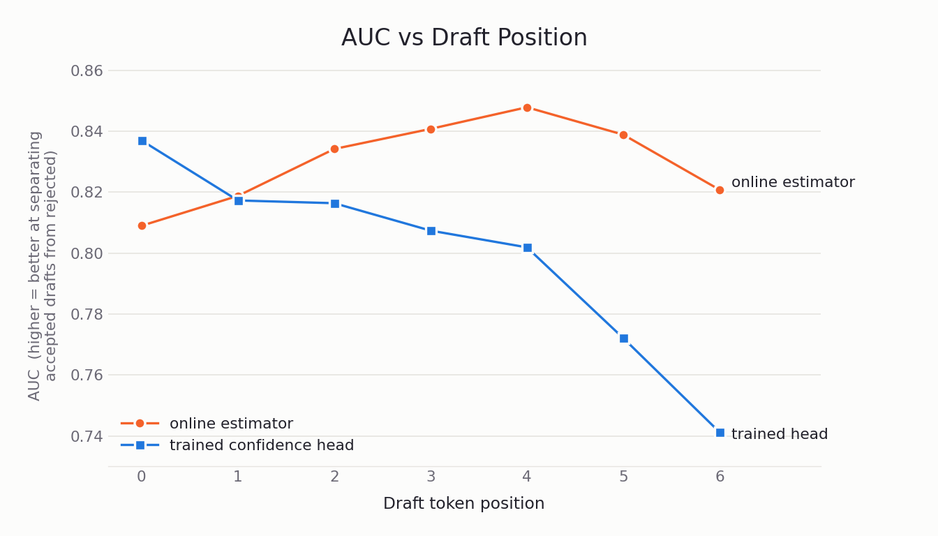
The confidence head is the better predictor on the first draft position, but the estimator takes the lead from the second position onwards. The gap widens with depth, with the estimator leading by 0.08 AUC by the last position. Both predictors also fall off after the fifth position. This is likely because DSV4-Flash's DSpark declares a block size of 5 and the drafter was never trained past it, so the drafts themselves get worse there.
Since survival is a running product, and the first draft position always carries a request's highest score, it is less often the token that the budget cuts. The estimator's advantage sits right where the trimming happens, and it explains why the estimator can match the confidence head in end-to-end performance.
Fitting the Coefficients
The coefficients ω and βi are continuously refitted during live serving of requests. Draft tokens proposed during the previous decode step are verified by the target model in the next decode step. Only draft tokens up until the first rejection (if any) are eligible for training on, because the target model has explicitly labeled them (accept or reject).
We use Iteratively Reweighted Least Squares (IRLS) to minimize the log-likelihood loss of the predictions vs the labels. This minimization is performed over a second-order Taylor approximation of the log-likelihood loss. The optimization step for ω and βi is obtained by solving the system of equations
$$ \mathbf{H} \Delta\boldsymbol{\theta} = -\mathbf{g} $$
where Δθ is the delta for the shared slope ω and the per-position intercepts βi, H is the Hessian of the loss function with a shape of (K + 1) × (K + 1), and g is the gradient of the loss function, with a size of K + 1.
A refit happens after every fixed round of N decode steps. During each decode step in that interval, we accumulate the Hessian and gradient values, which are derived from the coefficients, features, and labels collected during the round. Doing this upper bounds memory to O(K²) across a round, in contrast with O(N × B × K) if we instead collected the raw labels. On the final step of the round, the system is solved, and the coefficients are updated.
As one might expect, deeper drafts are accepted less often than shallower drafts. Consequently, deeper draft positions can be starved of labels during a round. Two design decisions were made to mitigate the impact of this on the refitting process:
- Shared Slope: The slope is shared across all draft positions to prevent noisy updates caused by data thinning at depth. Predictions are much more sensitive to slope errors than intercept errors, so sharing makes the Newton step well-determined. Furthermore, empirical measurements show sharing the slope costs virtually nothing in terms of accuracy (only 0.0002 AUC and 0.0003 log-loss).
- Step Damping: Each coefficient's update is scaled by the amount of supporting evidence using the formula n / (n + constant), where n is the count of graded drafts. This ensures that deeper positions with fewer labels move more conservatively, preventing updates based on noise.
Slope vs Intercept Roles
The fitted coefficients were tracked across several model/dataset combinations, and the two kinds of parameters behave very differently.
Hold the model pair fixed and vary the workload: Fitting DSV4-Flash + DSpark independently on each of five workloads, the slope barely moves (0.51 to 0.55), uncorrelated with how hard the workload is (r = −0.08 against mean draft entropy). The intercepts do the opposite: the first draft position intercept correlates with draft entropy at r = −0.89, and runs from ~0.5–0.6 on the more predictable workloads down to below 0 on the least.
| Dataset | Acceptance Rate | Mean Draft Entropy | Slope ω | Intercept β0 |
|---|---|---|---|---|
| gsm8k | 0.781 | 0.562 | 0.5365 | +0.478 |
| humaneval | 0.751 | 0.669 | 0.5135 | +0.486 |
| speed-bench 2k low-entropy | 0.755 | 0.703 | 0.5087 | +0.610 |
| mt-bench | 0.714 | 0.800 | 0.5495 | +0.181 |
| speed-bench 2k high-entropy | 0.642 | 1.077 | 0.5197 | −0.089 |
Now vary the model pair: The slope ranges from 0.45 to 0.59 across pairs, while staying tight within each one. The intercepts also differ between pairs, so unlike the slope they are not a property of one axis alone.
| Model | nspec | Slope ω | ω sd | Intercept β0 |
|---|---|---|---|---|
| DeepSeek-V4-Flash + DSpark | 5 | 0.5013 | 0.0250 | +0.279 |
| MiMo-V2.5-Pro-FP4 + DFlash | 8 | 0.5197 | 0.0415 | −1.000 |
| Inkling-NVFP4 + MTP | 8 | 0.5859 | 0.0349 | −0.572 |
| Muse-Glimmer-30B + DFlash2 | 7 | 0.4450 | 0.0323 | +0.167 |
Read together, the two tables suggest a division of labor. The slope measures how well the draft model knows when it's right. This is a property of the target/draft pair and the draft sampling method, which is why it barely moves when only the workload changes. The intercepts absorb the rest: the base acceptance rate at each draft position, which falls with depth and drops even further on less predictable content. That base acceptance rate depends on the model pair as well as the workload, which is why the intercepts move along both axes while the slope moves along just one.
Benchmarks
We benchmarked three checkpoints (MiMo-V2.5-Pro-FP4 + DFlash, Inkling-NVFP4 + MTP, and Muse-Glimmer-30B + DFlash2) that previously could not use AV at all, along with DSV4-Flash + DSpark + the estimator, and DSV4-Flash + DSpark + the confidence head, as a reference. The gains below were captured with AV off vs on, temperature 1.0, top-p 0.95, and concurrency 64, over four datasets.
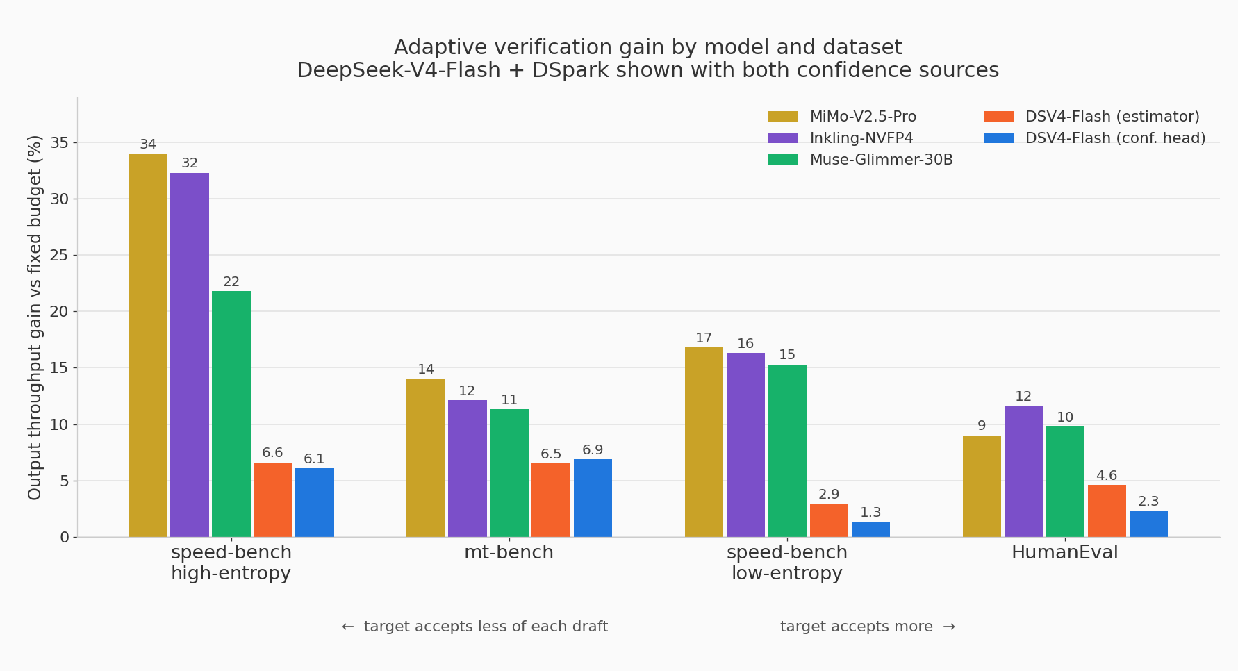
Compared to fixed verification, the online estimator at the same speculative length is a win across all benchmarked datasets. However, that gain alone doesn't tell the whole story. Oftentimes, a smaller fixed length can be found to outperform AV at the max speculative length at specific concurrencies. The Pareto curve below was captured with DSV4 + DSpark across a sweep of fixed speculative lengths and AV at the max speculative length:
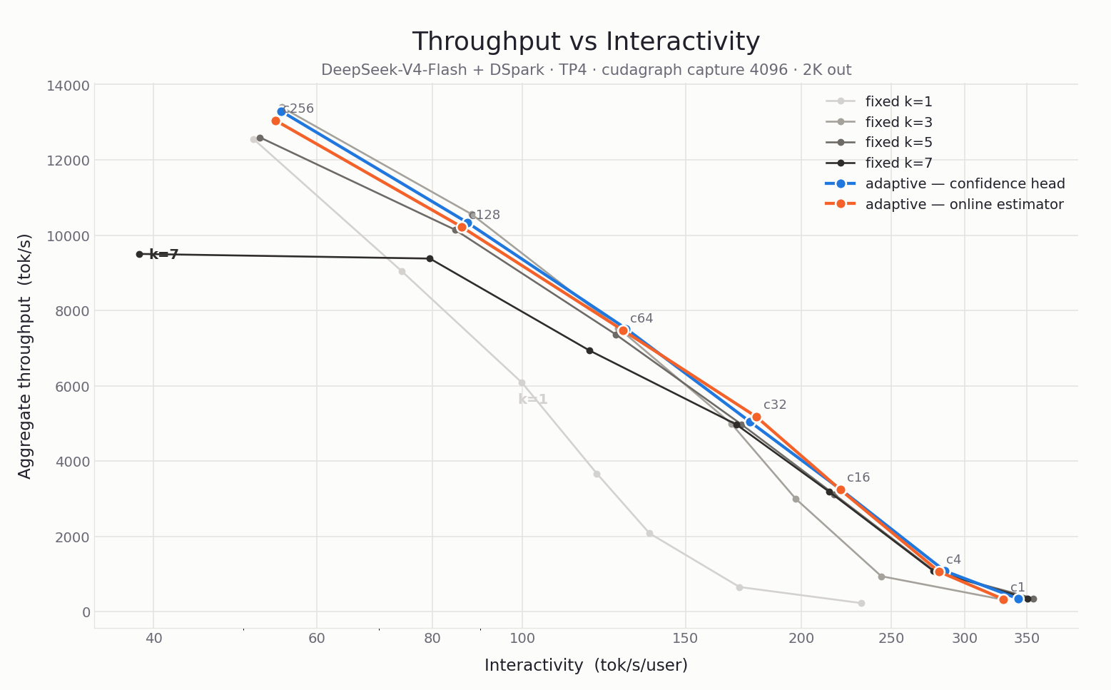
The online estimator and the confidence head are roughly on par in terms of performance, across all measured concurrencies. However, the online estimator is not meant to be a replacement for the confidence head, but rather a drop-in alternative in the absence of one. Let's see how it performs on a model pair that currently lacks a confidence head. Below is the Pareto curve for MiMo-V2.5-Pro-FP4 + DFlash across a sweep of fixed speculative lengths and AV:
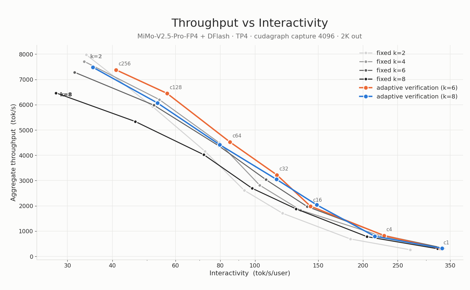
AV sits on the throughput-interactivity frontier at 5 of 7 concurrencies.
Limitations
- The target model's attention backend must support variable-length verification. This is the same prerequisite that DSpark AV already has.
- MTP and EAGLE benefit less from AV than DFlash and DSpark do. This is because those auto-regressive speculators pay a proportionally larger cost for drafting tokens that may get trimmed before verification.
vLLM Usage
AV is enabled through the speculative config. On a draft model that (1) has no confidence head and (2) supports variable length attention for all of its backends, the online estimator is selected automatically:
vllm serve <target_model> \
  ...
  --speculative-config '{
    "model": "<draft_model>",
    "method": "<method>",
    "num_speculative_tokens": <num_speculative_tokens>,
    "draft_sample_method": "probabilistic",
    "enable_adaptive_verification": true
  }'
Acknowledgements
This work was done by Giancarlo Delfin (Inferact), and builds directly on Adaptive Verification by Lucas Wilkinson (Red Hat) and Benjamin Chislett (NVIDIA).
[^1]: An example with a simple two-token vocabulary of [a, b] can be used to illustrate this bias. Assume p = [0.5, 0.5], q = [0.2, 0.8], and that a draft token is trimmed from verification if q(x) < 0.5. Drawing a results in trimming, and the target samples a token from its own distribution, p(x). However, drawing b results in verification: the token is accepted with probability min(1, p(b)/q(b)) = 0.625, and otherwise rejected and resampled from the residual norm(max(0, p − q)) = [1, 0], yielding a. During rejection sampling we get pout(a) = q(a)·p(a) + q(b)·(1 − 0.625) = 0.4 and pout(b) = q(a)·p(b) + q(b)·0.625 = 0.6. This differs from the target's distribution of [0.5, 0.5] and violates speculative decoding's lossless guarantee.